The mathematical description for multi-dimensional, steady-state heat-conduction is a second-order, elliptic partial-differential equation (a Laplace or Poisson Equation). Typical heat transfer textbooks describe several methods for solving this equation for two-dimensional regions with various boundary conditions. Analytical solutions usually involve an infinite series of transcendental functions. This series is truncated and evaluated at an array of locations to give an approximate estimate of the temperatures found over the 2-D region. Some texts also include detailed graphical methods using various paper and pen tools for estimating temperature and heat-flow lines for 2-D problems.
Module Description
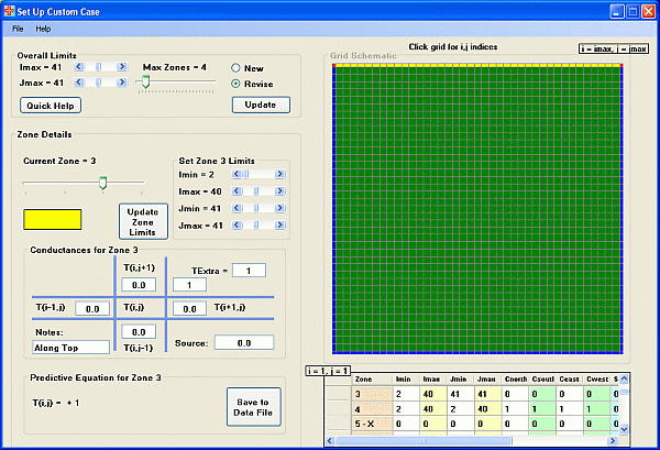
Inputs
n our software module, HTT_2dss, we employ modern numerical methods. Specifically the we use the finite-volume method, to solve for the temperature distribution over a user-specified 2-D region. The region is taken as rectangular, with cutouts possible. The user is asked to:
- specify the nodalization of the heat-conduction region. We use dynamic array allocation, so the problem size is limited only by the memory available.
- derive the appropriate heat-balance equations for specified regions of the solution domain (internal points, boundary edges, corners, interfaces, etc.), and
- input the resulting numerical coefficients on a special input form:
Calculations/Results
In doing this, they are (without knowing it) setting up the ranges of numerical Do-loops. The program then uses this input data to solve the large, sparse system of linear equations using a modern iterative technique known as the Modified Strongly Implicit Procedure. In just a few seconds, HTT_2DSS returns a full-color contour-plot of the resulting isotherms — for use in further analysis and verification. We present a sample of the main user-interface of HTT_2dss in the graphic below. The user may click anywhere on the contour plot to see the local heat flux vector (and experience firsthand the difference between vectors and scalars).

The user can also specify a raised contour plot:

Analytical Solutions
This main user-interface of Htt_2DSS includes easy access to two sample problems which have analytical solutions in the form of an infinite series. For these two samples the color-contour plot can be enhanced with the overlay of white lines depicting isotherms found using the analytical solution. The user may specify the number of terms to be used in the series approximation. (See also our Excel HTTtwodss spreadsheet which animates the analytical solution of one of these same sample problems by incrementally adding terms in the infinite series.)
Documentation
We have embedded several PowerPoint presentations within this module: One covers analytical solutions for two-dimensional conduction, including the graphical depiction of results. A second includes checking and interpreting numerical solutions. Meanwhile a third derives all needed governing heat balance equations. The fourth comprises a step-by-step tutorial for the case shown in the graphic above. Thorough instructions provide an even more thorough discussion of program operation, as well as the important physical and numerical aspects of this classical engineering problem.
Electrical Analogs
For this module and several others Mr. T.C. Scott developed desktop experiments from which the whole class takes data. Below we show an electric analog used to model steady-state conduction in a two-dimensional fin – thus reinforcing the idea of approximating a continuous system by a “lumped” one. The brown resistors represent conductive resistance between adjacent cells. The turquoise ones represent the convective resistance between the fin and the ambient air. Before digital computers, electrical analogs like this were a staple of heat transfer laboratories. For 3D problems such analogs could involve thousands of resistors all carefully soldered together.
We restrict this module to quite regular two-dimensional regions. Large, highly developed thermal analysis codes like CINDA in the hands of a skilled thermal analyst apply the same principles to complicated geometries such as the inside of an engine compartment and the innards of computers.

Video Introduction
Link to 5:05 minute YouTube introduction to the HTT_2dss program.
Software Availability
Copies of our HTT_2dss module are available for use as freeware at educational institutions.
Notice to International Users (where decimal points (periods) are used instead of commas to break up long numbers). If this module does not work properly, please change the language setting to English (US).
Other Software in the HTT Collection for 2D, Steady-State Conduction:
- Evaluation and animated display of the analytical solution for a 2D, SS example problem
- Conduction Shape Factors