Internal Forced Flow (Pipe Flow)
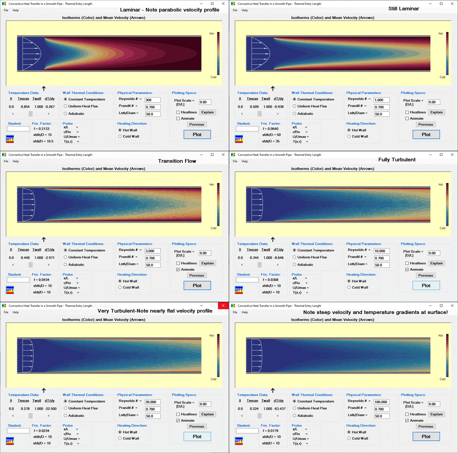
Heat transfer analysts usually handle internal (pipe) flows using convection correlations. For laminar flows the correlations are based on analysis; for transition and turbulent flows they are generally based on experiment. Another “on-screen” laboratory, our internal flow module instead solves the fundmental energy balance equation directly. Here we address the thermal entry length problem. In this scenario the velocity profile is already fully developed when a change in the wall thermal boundary condition is introduced. Our model handles laminar, transition and turbulent flows. The thermally (and hydrodynamically) fully developed condition is, of course, the asymptotic limit of the thermal entry problem.
The user of this “laboratory” selects either a fixed wall temperature or prescribed wall heat flux. To solve the discretized form of the governing advection-diffusion equation, our algorithm uses a single pass, space-wise marching technique. That scheme is implicit in the radial direction and is combined with backward differencing in the axial direction.
Module Description
Inputs
Inputs to the model include the Prandtl number of the fluid, the Reynolds number based on diameter, the Length/Diameter ratio for the pipe. The user selects whether a constant wall temperature or constant heat flux is applied to the surface. In addition, the user can specify a radial magnification factor for the display so that steep gradients can be observed more easily.
Display
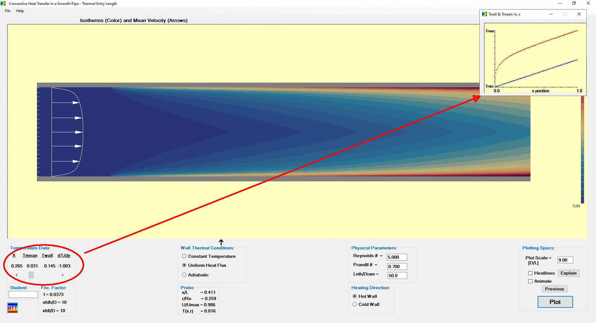
The calculation returns the temperature distribution as a function of axial location and radius in the form of a color contour plot. The results window also displays the velocity profile. The latter is unchanging, of course, since we assumed in this model that the flow is hydrodynamically fully developed. An option to display “Heatlines,” the convection heat transfer analog of streamlines, is available. Using a scrollbar (just to the bottom left of the contour plot in the screenshot below) the user can take data from the screen. This data includes the wall temperature, mixed mean temperature and the surface temperature gradient as a function of axial position along the pipe.

Measurements
Using the scrollbar data with an integral heat balance on a short length of the pipe or the latter directly, the user can develop a local or overall correlation for Nusselt number. The user can also use the mouse as a probe and “measure” local values of velocity and temperature. For values of Reynolds number greater than critical, the display gives the user the illusion of turbulence (the “fuzz” seen below).


Insights/Parameter Studies
Like the external flow module, this simulation allows an infinite number of flow and fluid input parameters. In addition, there is virtually no setup time and no hazardous materials! Using either of these forced flow modules the user becomes immediately aware of the tremendous difference in the heat transfer characteristics of various fluids. Ordinary (Pr = ~ 1.0) and extreme Prandtl number fluids (liquid metals Pr << 1 and oils (Pr >>1) behave very differently. Now the user can see physically the reason why. The user can explore the conditions under which the use of heat transfer enhancement techniques (surface roughening, turbulence promoters, etc.) might be justified.
To highlight the versatility of HTTpipe and encourage the testing of a wide range of parameters, we provide this secondary form to show the specific conditions to which the model is applicable:

Related Excel Workbooks
This Excel workbook implements conventional internal forced convection correlations. Note that the HTT_pipe module only applies to smooth pipes. An Excel workbook implementing conventional procedures for rough pipes is found here.
The Real Thing
The author of this module created it based on a lab experiment he did as an undergraduate engineering student a few years back:

The unheated starting section (where the velocity profile develops) is to the left. The heating begins roughly at the point along the pipe where the student sits. From that point on insulation covers the pipe surface.
Video Introduction to HTT_pipe module
Link to YouTube Introduction to HTT_pipe Video (3:40)
Reference
We describe the algorithm and present laminar flow results in: Ribando, R.J., and O’Leary, G.W., Numerical Methods in Engineering Education: An Example Student Project in Convection Heat Transfer,” Computer Applications in Engineering Education, Vol. 2, No.3, 1994, pp. 165-174. This article corresponds to the well-known Graetz (laminar flow) problem. It does not include the mixing length model used in the transition and turbulent regimes.
Notice to International Users (in those countries where decimal points (periods) are used instead of commas to break up long numbers). If does not work properly, then in the International Setting of the Windows Control Panel, please change the language to English (US).
